The visualization shows a Bayesian two-sample t test, for simplicity the variance is assumed to be known. It illustrates both Bayesian estimation via the posterior distribution for the effect, and Bayesian hypothesis testing via Bayes factor. The frequentist p-value is also shown. The null hypothesis, H0 is that the effect δ = 0, and the alternative H1: δ ≠ 0, just like a two-tailed t test. You can use the sliders to vary the observed effect (Cohen's d), sample size (n per group) and the prior on δ.
The prior on the effect is a scaled unit-information prior. The black, and red circle on the curves represents the likelihood of 0 under the prior and posterior. Their likelihood ratio is the Savage-Dickey density ratio, which I use here to compute the Bayes factor. The p-value is the traditional p-value for a two-sample t test with known variance (i.e. a Z test). HDI is the posterior highest density interval, which in this case is analogous a credible interval. And CI is the traditional frequentist confidence interval.
Have any suggestion? Or found any bugs? Send them to me, my contact info can be found here.